Toy Models
Here are a few models used to demonstate the package functionalities.
Forward Models
Lorenz
See https://en.wikipedia.org/wiki/Lorenz96model
using ECCO, CairoMakie
xyz=Lorenz_models.L96()
lines(xyz[1,:],xyz[2,:],xyz[end,:])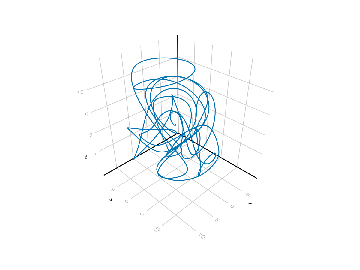
x,y,z=Lorenz_models.L63()
lines(x,y,z)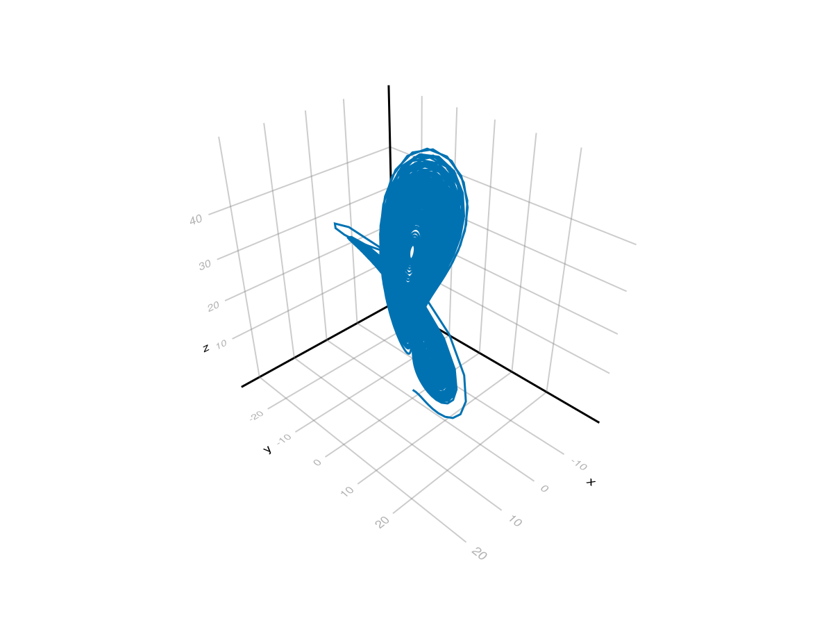
Budyko-Sellers Energy Balance Model
See this tutorial for detailed explanations.
using ECCO, Enzyme, Zygote, OrdinaryDiffEq, CairoMakie

(; Q, y) = Budyko_Sellers_models.params
Tsol,Tini,dTdt_ini,incr_t,incr=Budyko_Sellers_models.dTdt_demo(Q)

fig=Figure()
Axis(fig[1,1]); lines!(y,dTdt_ini)
Axis(fig[2,1]); lines!(y,Tini); lines!(y,Tsol,color=:red)
Axis(fig[3,1]); lines!(incr_t,incr)
fig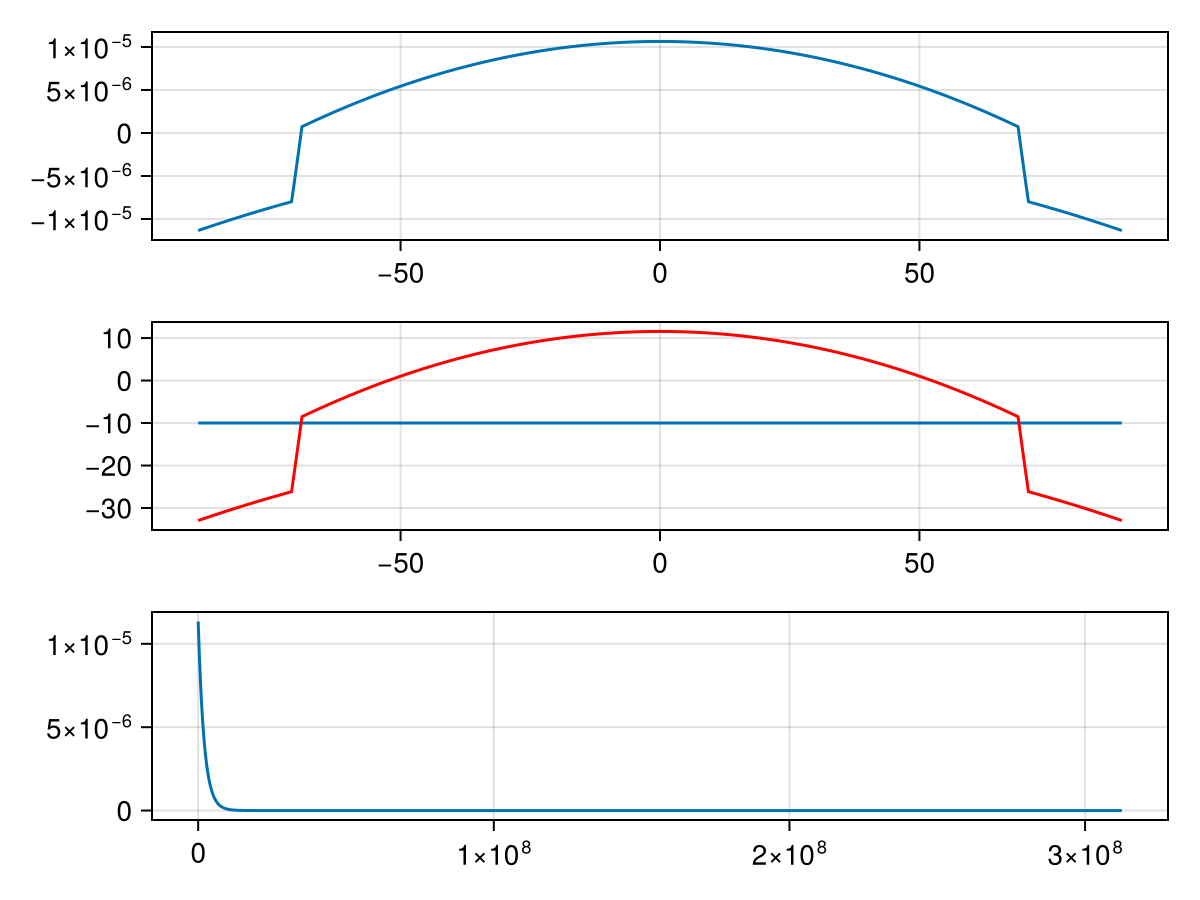
Parameter Choices
From B. Rose notebook :
R = 10^7 J/m2/K
From Walsh and Rackauckas :
- Figure 3. Equilibrium solutions (7) with albedo function (9) for five η-values. Note T∗ ηi (ηi) = Tc only for i = 2,5.
- Parameters: Q = 343, A = 202, B = 1.9, C = 3.04, αw = 0.32, αs = 0.62, Tc =−10.
- Figure 9. Equilibrium solutions of (2) with albedo function (34). Solid: η= 0.1. Dashed: η= 0.25. Dash-Dot: η= 0.4.
- Parameters: Q = 321,A = 167,B = 1.5,C = 2.25,M = 50,αw = 0.32,αi = 0.46,αs = 0.72,ρ= 0.35.
Earlier Implementations
- https://brian-rose.github.io/ClimateLaboratoryBook/courseware/one-dim-ebm.html
- https://github.com/ECCO-Summer-School/ESS25-Team_FLOW
- https://www.cise.ufl.edu/~luke.morris/2_4_2025/build/bsh/budyko_sellers_halfar/
Related References
- discrete and continuous – on the Budyko-Bellers energy balance climate model with ice line coupling – James Walsh, Christopher Rackauckas – doi:10.3934/dcdsb.2015.20.2187
- Theory of Energy-Balance Climate Models – Gerald R. North – 1975 – DOI: <https://doi.org/10.1175/1520-0469(1975)032<2033:TOEBCM>2.0.CO;2>
- Predictability in a Solvable Stochastic Climate Model – Gerald R. North and Robert F. Cahalan – DOI: https://doi.org/10.1175/1520-0469(1981)038%3C0504:PIASSC%3E2.0.CO;2
Glacier
Simple, 1D mountain glacier model inspired from the book Fundamentals of Glacier Dynamics, by CJ van der Veen, and which was translated to Julia by S Gaikwad.
See https://sicopolis.readthedocs.io/en/latest/AD/tutorial_tapenade.html#mountain-glacier-model
using ECCO, OrdinaryDiffEq
V=glacier_model.forward_problem(0.002)4.001702814498028Adjoint Calculations
Simple air-sea flux calculation
Simple air sea flux calculation and it's adjoint, obtained via Enzyme.
using ECCO, Enzyme, Zygote, OrdinaryDiffEq

ad=toy_problems.Enzyme_ex1()
println("x=$(ad.x) adfx=$(ad.adx)")
x=0.0 adfx=((3.858024691358025e-6,),)Bulk formulae
Air sea flux calculation derived using standard bulk formulae algorithm, and it's adjoint, obtained via Enzyme.
ad=toy_problems.Enzyme_ex2()
println("x=$(ad.x) adfx=$(ad.adx)")
x=(1.0, 10.0) adfx=((1.2244888899523058e-9, 8.970050297237849e-11),)ad=toy_problems.Enzyme_ex3()
println("x=$(ad.x) adfx=$(ad.adx)")x=([300.0, 0.001, 1.0, 10.0], [0.00915548218468587]) adfx=[0.0, 0.0, 0.01831096436937174, 0.0]ad=toy_problems.Enzyme_ex4()
println("x=$(ad.x) adfx=$(ad.adx)")x=([300.0, 0.001, 1.0, 10.0], [-3.0606099804357885]) adfx=[0.0, 917.7850566361462, -6.121219960871577, -0.44841281435892]ad=toy_problems.ForwardDiff_ex1()
println("x=$(ad.x) adfx=$(ad.adx)")x=[300.0, 0.001, 1.0, 10.0] adfx=[0.0, 458.8925283180731, -3.0606099804357885, -0.22420640717946003]ad=Zygote_examples.Zygote_ex1()ECCO.adjoint_result([300.0, 0.001, 1.0, 10.0], [0.0, 458.8925283180731, -3.0606099804357885, -0.22420640717946])Optimization Examples
using ECCO, Enzyme
op=toy_problems.optim_ex1()
op=toy_problems.optim_ex2()
op=toy_problems.optim_ex3()
ECCO.optim_result(ECCO.toy_problems.var"#h#optim_ex3##0"(), ECCO.toy_problems.var"#h!#optim_ex3##1"{ECCO.toy_problems.var"#h#optim_ex3##0"}(ECCO.toy_problems.var"#h#optim_ex3##0"()), [0.0, 0.0], [1.0000000001101883, 1.0000000002134781], * Status: success
* Candidate solution
Final objective value: 1.690037e-20
* Found with
Algorithm: L-BFGS
* Convergence measures
|x - x'| = 2.17e-08 ≰ 0.0e+00
|x - x'|/|x'| = 2.17e-08 ≰ 0.0e+00
|f(x) - f(x')| = 1.41e-15 ≰ 0.0e+00
|f(x) - f(x')|/|f(x')| = 8.35e+04 ≰ 0.0e+00
|g(x)| = 2.98e-09 ≤ 1.0e-08
* Work counters
Seconds run: 0 (vs limit Inf)
Iterations: 27
f(x) calls: 45
∇f(x) calls: 45
∇f(x)ᵀv calls: 0
)